Itamar Syn-Hershko
HNSW vs IVFFlat comparison: recall, memory, build time, and write workloads. Decision rules, parameter tuning, and examples.

HNSW and IVFFlat are two implementations of indexes for approximate vector search, often referred to as ANN (Approximate Nearest Neighbor).
HNSW is a graph-based vector index that reaches 95%+ recall out of the box and absorbs inserts without rebuilds, but uses 2-5x more memory than IVFFlat. IVFFlat partitions vectors into k-means Voronoi cells, builds faster, and uses less memory, but its recall drifts as data changes. Choose HNSW for most workloads under ~10M vectors with active writes; choose IVFFlat for very large, mostly static datasets where memory or build time dominates.
That summary is the answer most teams need. The rest of this post explains how the two algorithms work, what their parameters actually do, where each one fails, and how to make the call on real workloads. The comparison is at the algorithm level - pgvector is the worked example because it exposes both indexes through the same SQL surface, but the same tradeoffs show up in Milvus, Qdrant, Weaviate, OpenSearch, FAISS, and Pinecone.
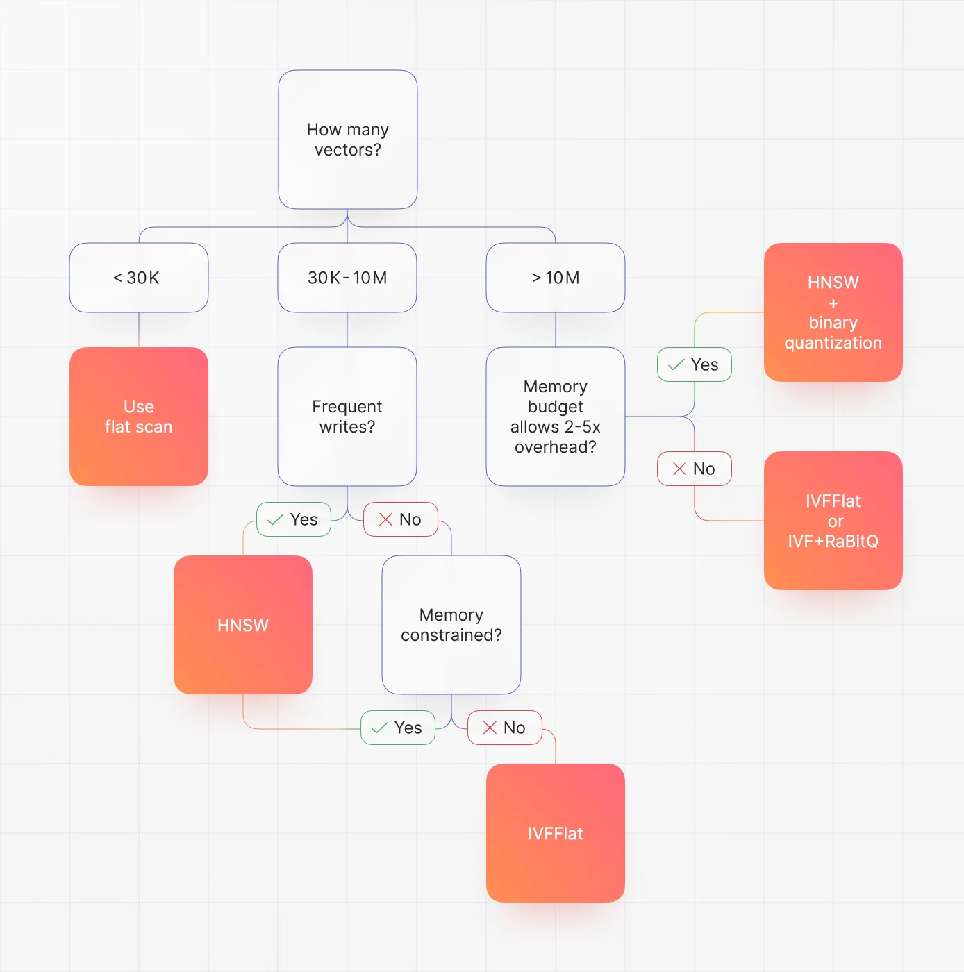
Quick decision flow
- Data changes often and recall matters: HNSW.
- Memory is tight and the dataset is past 50M vectors: IVFFlat.
- You need extreme memory efficiency: IVF + product or binary quantization (IVFPQ, IVF + RaBitQ).
What problem do vector indexes solve?
Vector search is performed via the nearest-neighbor algorithm, which is basically asking: given this vector, what are the vectors that are closest to it in distance and direction?
Exact nearest-neighbor search is O(n * d). With 100k+ vectors at 1536 dimensions (the size of OpenAI text-embedding-3-large outputs), a sequential scan blows past any real-time latency budget. pgvector falls back to a sequential scan when no index exists; FAISS exposes the same behaviour as IndexFlatL2. Recall is perfect, but you cannot run production traffic against it past a few tens of thousands of rows.
Approximate Nearest Neighbor (ANN) algorithms trade a small, controllable amount of recall for orders of magnitude in speed. Both HNSW and IVFFlat are ANN strategies. Neither guarantees exact results. Recall is measured as (retrieved ∩ true_top_k) / k, and production targets are typically 0.95 or higher.
Where this fits in the stack: an embedding model (OpenAI, Cohere, Voyage, Vertex, a local sentence-transformer) produces 768 to 3072-dimensional vectors that land in a vector index. The index choice directly shapes retrieval quality, which in a RAG pipeline cascades into the LLM's response quality. Get the index wrong and you get worse answers, not just slower ones.
How IVFFlat works
IVFFlat is short for Inverted File with Flat compression. At build time, k-means clusters the entire dataset into a fixed number of cells, each defined by a centroid. These cells are commonly called Voronoi cells: every point in vector space belongs to the cell whose centroid is closest. Each vector is assigned to exactly one cell, and the vectors inside a cell are stored uncompressed - that is what the "Flat" means. IVFPQ and IVF + RaBitQ replace this flat storage with quantized representations to save memory.
At query time, the index computes the distance from the query vector to every centroid, picks the closest few cells, and only scans the vectors in those cells. The number of cells visited is the probes parameter (sometimes nprobe). Few probes mean fast, lower-recall queries; more probes climb the recall curve at the cost of latency.
The architectural weakness sits at the build step. Cluster boundaries are decided once, when you run CREATE INDEX. They reflect only the data present at that moment. If you build on a partial or unrepresentative sample, your cells are skewed and recall stays bad until you rebuild. Best practice is to populate the table with at least 50k-100k representative vectors before issuing the build.
Inserts work, but new vectors are pushed into whichever existing cell has the nearest centroid. They cannot create new clusters or rebalance existing ones. As your data distribution drifts, recall degrades. The standard pattern is scheduled full rebuilds, weekly or monthly, tied to ingest rate and observed recall on a held-out query set.
Implementations to know:
- pgvector:
USING ivfflat,listsbuild parameter,ivfflat.probesquery parameter. - FAISS:
IndexIVFFlat, the canonical reference implementation. - Milvus:
IVF_FLAT, plus quantized variantsIVF_SQ8,IVF_PQ. - OpenSearch / Lucene: does not ship IVFFlat. HNSW only.
How HNSW works
HNSW stands for Hierarchical Navigable Small World, introduced by Malkov and Yashunin in 2016. The structure is a hierarchical graph. The top layer is sparse and contains a few "highway" nodes with long-range edges that let the search jump across the dataset quickly. Each lower layer is denser, with more nodes and shorter edges. The bottom layer holds every vector with high-precision local connectivity. Nodes are assigned to layers using an exponentially decaying probability, so a tiny fraction of vectors live at the top, and most live near the bottom.
Construction inserts one vector at a time. For each insert, HNSW runs a best-first search of width ef_construction to find the new node's approximate nearest neighbors, then wires it up with at most m edges per layer. Higher m produces a denser graph - better recall, more memory. Higher ef_construction produces a better-quality graph at the cost of build time. pgvector 0.6.0 (January 2024) added parallel HNSW builds, which cuts wall-clock build time substantially on multi-core machines.
Queries enter at the top layer, greedily follow long-range edges toward the query vector, then descend layer by layer with progressively finer search. The ef_search parameter controls the candidate list width during traversal. Time complexity is O(log n), which is why HNSW scales gracefully where IVFFlat's O(probes * cluster_size) starts to bite.
The single most useful property for production: HNSW absorbs inserts without quality loss. The graph adapts as nodes arrive. There is no rebuild step, no maintenance window, no recall drift. Deletes are handled by tombstoning, with optional compaction. That is why every modern vector database (Milvus, Qdrant, Weaviate, Pinecone, OpenSearch) defaults to HNSW.
Implementations to know:
- pgvector:
USING hnsw, withmandef_constructionbuild params,hnsw.ef_searchquery param. - FAISS:
IndexHNSWFlat. - hnswlib: the canonical C++ reference; used internally by Weaviate and Qdrant.
- Lucene / OpenSearch / Elasticsearch: Lucene HNSW, a Java port.
- Milvus, Qdrant, Weaviate, Pinecone: all default to HNSW for similarity search.
Head-to-head comparison
| Dimension | HNSW | IVFFlat |
|---|---|---|
| Index type | Graph-based, hierarchical | Inverted-file partitioning (k-means) |
| Build time (1M vectors) | Minutes to hours | Seconds to minutes |
| Memory overhead | ~2-5x raw vectors | ~1.1x raw vectors |
| Default recall | 95%+ out of the box | Depends heavily on lists/probes |
| Write resilience | Excellent, no rebuild needed | Drifts; periodic rebuild required |
| Query latency scaling | O(log n) |
O(probes * cluster_size) |
| Best for | Dynamic data, RAG, semantic search | Very large + mostly static datasets |
| Tuning surface | m, ef_construction, ef_search |
lists, probes |
A few concrete data points anchor the table. On the AWS pgvector benchmark at roughly 58k records and 1536 dimensions on a db.r5.large RDS instance, IVFFlat built in about 15 seconds and HNSW in about 81 seconds on pgvector 0.5.0. With pgvector 0.6.0's parallel builds, the same HNSW build dropped to about 30 seconds. Query latency on the same workload landed around 1.5ms for HNSW and 2.4ms for IVFFlat, both far ahead of the 650ms sequential scan. These are illustrative numbers on a small dataset and a small instance - run your own benchmarks before committing to a configuration.
Memory is where IVFFlat genuinely wins. HNSW stores neighbor lists at every layer, so the graph itself can run 2-5x the size of the raw vectors. IVFFlat stores centroid metadata plus flat per-cell vector lists, which is much closer to 1x the raw data. At 50M+ vectors with 1536 dimensions, the gap can be tens of gigabytes of RAM. Recent pgvector releases - 0.7.0 added binary_quantize, halfvec, and sparsevec; 0.8.0 added iterative scans - close most of this gap by combining HNSW with binary quantization, at a small recall cost.
Write performance is where HNSW wins, decisively. Inserts are constant-cost graph operations and graph quality holds up. IVFFlat inserts are cheap too, but they are the source of recall drift, because the cell structure does not adapt. If your dataset is changing every hour and your maintenance window is "never", HNSW is not really a choice - it is the only option that does not require operational scaffolding for periodic rebuilds.
Tuning parameters in practice
IVFFlat: lists and probes
lists controls how many cells k-means produces. The standard rule of thumb:
- Up to 1M rows:
lists = rows / 1000. - Over 1M rows:
lists = sqrt(rows).
probes controls how many cells the query touches. Start at 1-10% of lists and increase until recall hits your target. Production values commonly land between 10 and 30.
CREATE INDEX ON items USING ivfflat (embedding vector_cosine_ops) WITH (lists = 1000);
  SET ivfflat.probes = 10;
HNSW: m, ef_construction, ef_search
The pgvector defaults (current as of 0.8.2) are:
m = 16: max connections per node.ef_construction = 64: build-time candidate list width. Should be at least2 * m.ef_search = 40: query-time candidate list width.
Tuning guidance:
- Higher
m(up to ~48) raises recall and roughly linearly raises memory. - Higher
ef_construction(up to ~256) improves graph quality at the cost of slower builds. - Higher
ef_search(80-200) raises recall at the cost of latency.
CREATE INDEX ON items USING hnsw (embedding vector_cosine_ops) WITH (m = 16, ef_construction = 64);
  SET hnsw.ef_search = 100;
The right parameter set depends on data shape, query patterns, and latency budget. Treat the defaults as a sane starting point, not a final answer.
Validating recall
Build a labelled query set of 100-500 queries with known ground truth. The cheapest way to generate ground truth is to run the same queries against a flat (exact) index. Then compare top-K overlap between the indexed query and the exact result. Wire this into CI so that index changes, version upgrades, and parameter tuning are validated against a recall floor before they hit production.
Disk vs RAM
IVFFlat tolerates partial disk residency reasonably well. Cells localize access, and reading a single cell is mostly sequential. HNSW expects most of the graph in RAM. Cold queries against an on-disk HNSW index can be brutally slow because every traversal step is a potential page fault. pgvector 0.8.0 improved this with iterative scans and better on-disk HNSW handling, but the rule of thumb still holds: budget for the graph in memory if you want predictable latency.
Decision framework
Use HNSW when
- Dataset is under roughly 10M vectors and memory is not severely constrained.
- Data changes frequently. Continuous inserts, updates, deletes are the norm.
- You need 95%+ recall, especially in RAG or semantic search where missed context degrades downstream answers.
- You want a "set and forget" index with no rebuild scheduling.
- You are starting fresh and do not yet have benchmarks for your data distribution.
Use IVFFlat when
- Dataset is very large (50M+ vectors) and the memory budget is tight.
- Data is static or you can schedule periodic rebuilds during maintenance windows.
- Build time is itself a critical constraint: frequent reindexing in CI/CD, batch ML pipelines, regulated environments where indexes are rebuilt nightly.
- You can populate the table with a representative sample before the k-means build.
The crossover region
- Below ~30k vectors: a flat scan is often acceptable. Single-digit milliseconds at 1536 dimensions on modern hardware.
- 30k-50k: switching to HNSW gives noticeable recall and latency improvements.
- Above 50k: HNSW is the default unless memory or dataset-size constraints push you to IVFFlat.
pgvector as the canonical example
pgvector exposes both indexes with the same SQL surface, which makes it the easiest stack to test the choice on your own data. pgvector 0.8.2 (February 2026) is the current release and supports HNSW, IVFFlat, halfvec, sparsevec, and binary quantization. The same algorithmic tradeoffs apply across Milvus, Qdrant, Weaviate, OpenSearch, FAISS, and Pinecone - only the parameter names and operational surface change. We covered scaling these systems further in our vector search scaling guide and the OpenSearch vector search introduction.
What's next: quantized indexes
The HNSW memory disadvantage is shrinking, fast. pgvector 0.7.0 added binary_quantize, which collapses each dimension to a single bit. Combined with HNSW, this produces a graph that is small enough to keep in RAM at scales where flat HNSW would not fit, with a modest recall cost that is acceptable for most RAG workloads. Recent benchmarks suggest very large p99 latency improvements and dramatic build-time reductions versus IVFFlat at high recall targets, though the exact numbers vary by dataset and hardware - measure on your own data before committing.
IVF + RaBitQ is the other side of this trend. It pairs IVF partitioning with randomized binary quantization, aiming to deliver HNSW-like recall at IVFFlat-like memory cost. It is moving from research libraries into production engines including VectorChord and Milvus.
DiskANN and ScaNN sit further out. DiskANN is a graph index designed for SSD-resident operation. ScaNN focuses on high-recall, high-throughput inner-product search. Both are worth tracking as RAM costs become the dominant constraint for billion-scale vector search.
Frequently asked questions
What is the difference between ANN and HNSW?
ANN (Approximate Nearest Neighbor) is a category of search algorithms that trade a small amount of recall for large speedups over exact search. HNSW is one specific algorithm within that category - a multi-layer graph index. Other ANN algorithms include IVFFlat, IVFPQ, ScaNN, and DiskANN.
Does pgvector use HNSW?
Yes. pgvector supports both HNSW and IVFFlat. HNSW was added in pgvector 0.5.0 (August 2023) and is the recommended default for most pgvector workloads as of 2026.
How does the HNSW index work?
HNSW builds a hierarchical graph in which every vector is a node connected to its approximate nearest neighbors. Top layers contain sparse "highway" edges for long-range jumps. Lower layers have dense local connections. Queries enter at the top, greedily traverse highway edges toward the target, then descend into denser layers for fine-grained search. Query time is O(log n).
What is IVF in vector search?
IVF (Inverted File) is an indexing strategy that partitions vectors into clusters using k-means. At query time, only the closest few clusters - controlled by probes - are searched, which sharply reduces computation. IVFFlat stores raw vectors in each cluster. IVFPQ and IVF + RaBitQ add quantization for memory efficiency.
Is HNSW always better than IVFFlat?
No. HNSW dominates for most workloads under ~10M vectors with active writes, but IVFFlat is the right call when memory is tight, the dataset is very large (50M+) and mostly static, or build time matters more than query latency.
Can I switch from IVFFlat to HNSW without downtime?
Yes. Most engines support concurrent index creation. In Postgres/pgvector, CREATE INDEX CONCURRENTLY builds the new HNSW index in the background, and you drop the old IVFFlat index after the new one is online.
Key takeaways
- HNSW is the default for most production vector search workloads as of 2026: high recall, dynamic data, predictable scaling.
- IVFFlat earns its place when the dataset is very large, mostly static, and memory or build time dominates the cost model.
- pgvector exposes both indexes through the same SQL surface, which makes it the simplest place to evaluate the tradeoff on real data.
- HNSW defaults (
m=16,ef_construction=64,ef_search=40) are a sane starting point. Tuneef_searchfirst. - IVFFlat tuning is mostly about
lists(size at build time) andprobes(recall vs latency at query time). Plan for periodic rebuilds. - Binary quantization combined with HNSW is closing the memory gap. Watch IVF + RaBitQ, DiskANN, and ScaNN for billion-scale workloads.
If you are picking a vector index for a new system, start with HNSW. If your scale or memory budget tells you HNSW will not fit, IVFFlat is still a solid, well-understood option - just budget for the rebuild cadence from day one.