Itamar Syn-Hershko
The Apache Iceberg Table Format explained - a layer-by-layer walkthrough of catalogs, metadata files, manifest lists, manifests, and data files, with a concrete example of what happens on disk when you create and write to a table.

We first wrote about Apache Iceberg back in 2019, when it was still an early-stage open table format out of Netflix. We were convinced then that it would reshape how data warehousing works. That bet paid off - Iceberg is now the standard for data lakehouse architectures and has native support across every major cloud platform and query engine.
But most explanations stop at the feature list: ACID transactions, time travel, schema evolution. What does the iceberg table format actually look like on disk? How does a query engine go from a table name to the exact set of Parquet files it needs to scan? This post walks through the architecture layer by layer, then shows what happens in object storage when you create a table and write to it.
The Problem Iceberg Solves
Data warehouses worked well for decades - batch ETL overnight, controlled schemas, predictable query patterns. But they were expensive, proprietary, and locked your data into a single vendor's format. Data lakes swung the pendulum the other way: dump everything into a distributed file system (Hadoop initially, then S3), store it cheaply, figure out the schema later.
"Figure out the schema later" turned out to mean "lose the things that made warehouses reliable." Without a management layer above raw files, data lakes had no ACID guarantees, no schema tracking, and no consistent view of data during concurrent writes. If two writers touched the same table at the same time, you got lucky or you got corrupted data. Changing a partition layout meant rewriting everything. And the organizational side was just as bad: teams would ETL subsets of lake data into warehouses, then analysts would export CSVs from those warehouses onto their laptops, and suddenly five copies of the same data existed with no single source of truth. That's data drift, and it creates compliance and accuracy problems that are hard to even detect, let alone fix.
The data lakehouse model solves this by keeping everything on cheap object storage but organizing files into managed tables using an open table format like Iceberg. Instead of copying data into a proprietary system, you add iceberg metadata on top of Parquet files already sitting in S3 or GCS. Any engine that speaks Iceberg - Spark, Trino, Flink, Dremio, Athena - queries those tables directly. No extra copies. No format lock-in.
A data lakehouse built on Iceberg has five distinct components: object storage for files, a columnar file format (Parquet is the standard), the iceberg table format for the metadata layer, a catalog to track what tables exist, and one or more query engines to run operations on the data. Each is a separate choice, and each is swappable.
The Four Layers of Iceberg Metadata
Understanding the architecture comes down to understanding four layers stacked on top of data files, each serving a specific role in query planning and table management.
Data Files and Manifests
Data files are at the bottom. Regular Parquet, ORC, or Avro files - the same columnar files you'd have in any data lake. Nothing special about their format. They live in whatever storage you're using.
Manifest files sit above them. A manifest tracks individual data files, but it's not just a list of paths. Each entry records the file's storage location, its format, its partition values, the record count, and column-level statistics - specifically the lower and upper bounds for each column along with null counts. Those statistics are what allow engines to skip files during query planning without opening them. Say your query filters on age BETWEEN 20 AND 30. If a manifest entry says a file's age column ranges from 50 to 80, the engine drops that file immediately. No I/O wasted.
Manifest Lists and Metadata Files
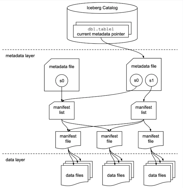
Manifest lists group manifests into snapshots. Each time the table changes, a new manifest list is created referencing all the manifests that belong to that version of the table. The key benefit here is partition-level pruning at the group level. If a manifest represents data partitioned by month and your query only needs June, the engine tosses out any manifest covering July without inspecting individual file entries inside it. This two-level pruning - first eliminate manifest groups, then eliminate individual files using column statistics - is why Iceberg query planning is so much faster than the old Hive approach of listing directories and scanning files one by one.
Metadata files hold the global table state. This is where the current schema lives, alongside an array of every previous schema version, each with an ID. Same for partition specs. Each snapshot in the metadata file references the schema ID and partition spec ID it was written with, so when the engine reads files written under an older layout, it knows exactly how to interpret them. The metadata file also maintains the full snapshot history: the current snapshot, all previous snapshots, each pointing to its own manifest list. This is what makes time travel work and what makes schema evolution safe - you never modify existing files, you just create a new snapshot that represents the current state.
The Catalog
Every query starts at the catalog. Think of it as a phone book: you look up a table name and get back the path to its current metadata file. The catalog itself doesn't store schemas or file lists - all of that lives in the metadata layer.
The catalog can be many things. A Hive Metastore, a JDBC-backed database, AWS Glue, Project Nessie, or an Iceberg REST Catalog endpoint. The one hard requirement is that it needs to support some form of atomic update, because when a writer commits a new snapshot, it atomically swaps the catalog's pointer from the old metadata file to the new one. That atomic swap is the mechanism that gives Iceberg its concurrency safety. You can technically use HDFS as a catalog - it'll read the table directory - but it's not recommended for production with multiple writers because it lacks the locking mechanism other catalogs provide.
So the full query path looks like this: engine asks the catalog for a table name, gets a metadata file path, reads the metadata file to find the current snapshot, follows the snapshot to its manifest list, prunes manifests by partition info, then drills into surviving manifests to prune individual files by column statistics. By the time the engine starts scanning actual data, it has the narrowest possible set of files. Different engines may exploit this metadata differently and optimize their scan differently on top of it, which is why engine choice still matters even when they're all reading the same iceberg table format.
What Actually Happens on Disk
Let's make this concrete. Say you run:
CREATE TABLE orders (
    order_id BIGINT,
    customer_id BIGINT,
    amount DECIMAL(10,2),
    order_date DATE
  );
Three things happen. A JSON metadata file is created in the table's metadata directory containing the schema, an initial snapshot (s0), and a reference to an empty Avro manifest list - because there's no data yet. The catalog entry for orders is set to point at this metadata file.
On S3, the resulting structure looks like:
orders/
    metadata/
      v1.metadata.json
      snap-0-<uuid>.avro
Now insert some records. A Parquet data file is written to the table's data directory. A manifest file (Avro) is created pointing to this data file, carrying the per-column statistics. A new manifest list (also Avro) is created pointing to that manifest. A new metadata file is created with a new snapshot (s1) that references the new manifest list while keeping a reference to s0. The catalog pointer atomically swaps to the new metadata file.
After the insert, S3 looks like:
orders/
    data/
      <uuid>.parquet
    metadata/
      v1.metadata.json
      v2.metadata.json
      snap-0-<uuid>.avro
      snap-1-<uuid>.avro
      <uuid>-m0.avro
Two JSON files for the two metadata versions. Two snap-prefixed Avro files for the manifest lists. One Avro manifest file. Every subsequent write follows the same pattern: create files bottom-up (data file, manifest, manifest list, metadata file), then swap the pointer at the top. Because the pointer swap is atomic and everything else is immutable, readers always see a consistent table state. That's ACID without a database.
Copy-on-Write vs. Merge-on-Read
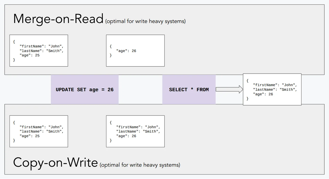
The immutable file model described above is clean in theory, but it raises an obvious question: what happens when you update or delete a single row? You can't edit a Parquet file in place. Iceberg gives you two strategies for handling row-level changes, and the choice has real consequences for read latency, write throughput, and table maintenance overhead.
Copy-on-Write (CoW) is the simpler approach. When a row is updated or deleted, Iceberg rewrites every data file that contains affected rows - producing new Parquet files with the changes applied - and points the new snapshot to those rewritten files. Reads stay fast because every file is always complete and self-contained; there's nothing to merge at query time. The cost lands entirely on writes. Rewriting a 1 GB file to change three rows is expensive, and write amplification compounds under any workload with frequent small updates. CoW is the right default for append-heavy pipelines or tables that are read far more than they're written.
Merge-on-Read (MoR) flips the trade-off. Instead of rewriting data files, Iceberg writes small delete files alongside the originals. Two kinds exist: positional delete files, which record the exact file path and row offset of each deleted row, and equality delete files, which record the values of one or more columns that identify rows to remove. The new snapshot references both the original data files and the new delete files. Writers pay almost nothing - appending a small Avro or Parquet delete file is orders of magnitude cheaper than rewriting a full data file. Readers pay the price: every scan must open surviving data files and apply the relevant delete files in memory before returning results. As delete files accumulate across many write operations, read overhead grows steadily.
The choice is a table-level configuration in Iceberg (write.delete.mode, write.update.mode, write.merge.mode), so you can mix strategies across tables in the same catalog depending on their access patterns. A CDC-ingested events table that receives constant row-level updates is a natural fit for MoR; a reporting table that receives nightly batch loads and is queried heavily throughout the day favors CoW. MoR tables need regular compaction to merge delete files back into full data files and restore read performance - which loops directly into the maintenance concerns that come with any Iceberg deployment.
Key Takeaways
Iceberg's architecture is a hierarchy: catalog → metadata file → manifest list → manifest → data file. Each layer enables a different level of query pruning, from partition-level group elimination down to column-level min/max filtering on individual files. Writers never modify existing files. They create new ones and atomically swap a single pointer. And because all of this is just JSON and Avro files in a bucket alongside Parquet data files, any engine that implements the spec can read and write the same tables.
The flip side is that this metadata layer needs maintenance. Snapshots accumulate, manifest files fragment, and small data files pile up over time. For practical guidance on compaction, snapshot expiry, and orphan file cleanup, see our post on Iceberg table maintenance best practices.